---
title: "Feature Selection: A linear regression approach to find the impact of the features of e-commerce sales data"
author: "Rafiq Islam"
date: "2022-08-30"
collection: portfolio
citation: true
search: true
lightbox: true
format:
html: default
ipynb: default
---
## Load the data
```{python}
import pandas as pd
import numpy as np
import seaborn as sns
import matplotlib.pyplot as plt
from mywebstyle import plot_style
plot_style('#f4f4f4')
salesdata = pd.read_csv('Ecommerce Customers')
salesdata.head()
```
## EDA
### Descriptive Statistics
```{python}
salesdata.describe()
```
```{python}
salesdata.info()
```
### Visualization
```{python}
fig, (ax1, ax2) = plt.subplots(1, 2, figsize=(7.9, 5))

# Scatter plot with regression line for 'Time on Website' vs 'Yearly Amount Spent'
sns.scatterplot(
    x='Time on Website', y='Yearly Amount Spent',
    data=salesdata, ax=ax1
    )
sns.regplot(
    x='Time on Website', y='Yearly Amount Spent',
    data=salesdata, ax=ax1, scatter=False, color='blue'
    )
ax1.set_title('Time on Website vs Yearly Amount Spent')

# Scatter plot with regression line for 'Time on App' vs 'Yearly Amount Spent'
sns.scatterplot(
    x='Time on App', y='Yearly Amount Spent',
    data=salesdata, ax=ax2
    )
sns.regplot(
    x='Time on App', y='Yearly Amount Spent',
    data=salesdata, ax=ax2, scatter=False, color='blue'
    )
ax2.set_title('Time on App vs Yearly Amount Spent')

plt.tight_layout()
plt.show()
```
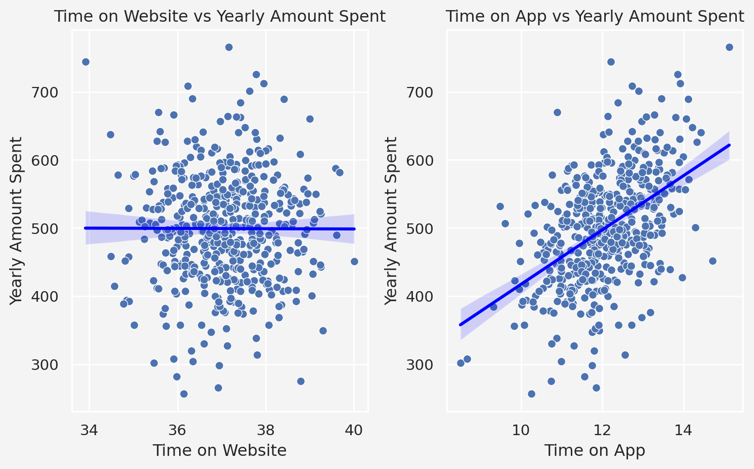
So, from this plot, we see that `Time on Website` has no significant trend or pattern on `Yearly Amount Spent` variable. However, `Time on App` seems to have a linear relationship on `Yearly Amount Spent`.
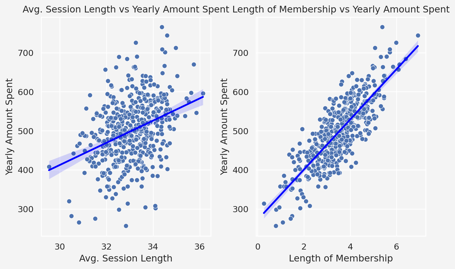
Next, we see the relationship between `Avg. Session Length` vs `Yearly Amount Spent`, and `Length of Membership` vs `Yearly Amount Spent`.
```{python}
fig, (ax1, ax2) = plt.subplots(1, 2, figsize=(7.9, 5))

# Scatter plot with regression line for 'Time on Website' vs 'Yearly Amount Spent'
sns.scatterplot(
    x='Avg. Session Length', y='Yearly Amount Spent',
    data=salesdata, ax=ax1
    )
sns.regplot(
    x='Avg. Session Length', y='Yearly Amount Spent',
    data=salesdata, ax=ax1, scatter=False, color='blue'
    )
ax1.set_title('Avg. Session Length vs Yearly Amount Spent')

# Scatter plot with regression line for 'Time on App' vs 'Yearly Amount Spent'
sns.scatterplot(
    x='Length of Membership', y='Yearly Amount Spent',
    data=salesdata, ax=ax2
    )
sns.regplot(
    x='Length of Membership', y='Yearly Amount Spent',
    data=salesdata, ax=ax2, scatter=False, color='blue'
    )
ax2.set_title('Length of Membership vs Yearly Amount Spent')

plt.tight_layout()
plt.show()
```
Both of these features have impact on the dependent variable. However, `Length of Membership` seems to have the most significant impact on `Yearly Amount Spent`.
```{python}
sns.pairplot(salesdata)
```
## Modeling
### Training
```{python}
from sklearn.linear_model import LinearRegression
from sklearn.model_selection import train_test_split

X = salesdata[
    ['Avg. Session Length', 'Time on App',
    'Time on Website', 'Length of Membership']
    ]
y = salesdata['Yearly Amount Spent']

X_train, X_test, y_train, y_test = train_test_split(
    X, y, test_size = 0.30, random_state=123
)

linreg = LinearRegression()
linreg.fit(X_train, y_train)
print('Coefficients: \n', linreg.coef_)
```
### Testing
```{python}
pred = linreg.predict(X_test)
plt.scatter(y_test, pred)
plt.xlabel('y test')
plt.ylabel('predicted y')
plt.show()
```
### Model Evaluation
```{python}
from sklearn import metrics

print('MAE', metrics.mean_absolute_error(y_test, pred))
print('MSE', metrics.mean_squared_error(y_test, pred))
print('RMSE', metrics.root_mean_squared_error(y_test, pred))
print('R-squared:', metrics.r2_score(y_test, pred))
```
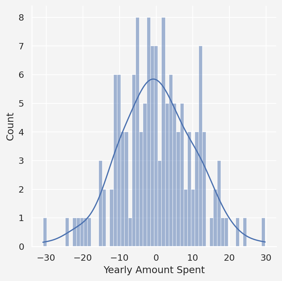
### Residual Analysis
```{python}
sns.displot(y_test-pred, bins= 60, kde=True)
```
## Conclusion
```{python}
coeff = pd.DataFrame({
    'Feature': ['Intercept'] + list(X.columns),
    'Coefficient': [linreg.intercept_] + list(linreg.coef_)
})

coeff
```