Insurance Cost Forecast by using Linear Regression

Author

Rafiq Islam

Published

September 12, 2024

Data Gathering, Defining Stakeholders and KPIs

Data Loading

import pandas as pd

insurance = pd.read_csv('insurance.csv')

insurance.sample(5, random_state=111)

	age	sex	bmi	children	smoker	region	charges
1000	30	male	22.99	2	yes	northwest	17361.7661
53	36	male	34.43	0	yes	southeast	37742.5757
432	42	male	26.90	0	no	southwest	5969.7230
162	54	male	39.60	1	no	southwest	10450.5520
1020	51	male	37.00	0	no	southwest	8798.5930

Exploratory Data Analysis (EDA)

Data Information

insurance.info()

<class 'pandas.core.frame.DataFrame'>
RangeIndex: 1338 entries, 0 to 1337
Data columns (total 7 columns):
 #   Column    Non-Null Count  Dtype  
---  ------    --------------  -----  
 0   age       1338 non-null   int64  
 1   sex       1338 non-null   object 
 2   bmi       1338 non-null   float64
 3   children  1338 non-null   int64  
 4   smoker    1338 non-null   object 
 5   region    1338 non-null   object 
 6   charges   1338 non-null   float64
dtypes: float64(2), int64(2), object(3)
memory usage: 73.3+ KB

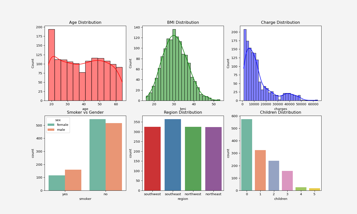
No missing data. Total 1338 observations.

Data Description

Statistical properties of the non-categorical variables

print(insurance.describe())

               age          bmi     children       charges
count  1338.000000  1338.000000  1338.000000   1338.000000
mean     39.207025    30.663397     1.094918  13270.422265
std      14.049960     6.098187     1.205493  12110.011237
min      18.000000    15.960000     0.000000   1121.873900
25%      27.000000    26.296250     0.000000   4740.287150
50%      39.000000    30.400000     1.000000   9382.033000
75%      51.000000    34.693750     2.000000  16639.912515
max      64.000000    53.130000     5.000000  63770.428010

Data visualization

Distribution of the features and target

import seaborn as sns
import matplotlib.pyplot as plt

fig, axes = plt.subplots(2,3,figsize = (15,9))

sns.histplot(insurance['age'], color='red', kde=True, ax= axes[0, 0]).set_title('Age Distribution')

sns.histplot(insurance['bmi'], color='green', kde=True, ax= axes[0,1]).set_title('BMI Distribution')

sns.histplot(insurance['charges'],color='blue', kde=True, ax= axes[0,2]).set_title('Charge Distribution')

sns.countplot(x='smoker', data=insurance, hue='sex', palette='Set2', ax=axes[1,0]).set_title('Smoker vs Gender')

sns.countplot(x=insurance['region'], hue=insurance['region'], palette='Set1', ax=axes[1,1]).set_title('Region Distribution')

sns.countplot(x=insurance['children'], hue=insurance['children'],legend=False,palette='Set2', ax=axes[1,2]).set_title('Children Distribution')

plt.gcf().patch.set_facecolor('#f4f4f4')

Data Vizualization

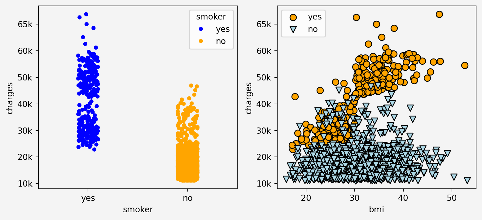
Relationship of the features and target

fig, axes = plt.subplots(1,2, figsize=(9.5,4))
g=sns.stripplot(data=insurance, x='smoker', y='charges', hue='smoker' ,palette=['blue', 'orange'], legend=True, ax=axes[0])
g.set_yticklabels(['0k','10k','20k','30k','40k','50k','60k','65k'])

axes[1].scatter(insurance.loc[insurance.smoker=='yes'].bmi,
            insurance.loc[insurance.smoker=='yes'].charges, label="yes", marker='o',
            s=60,edgecolors='black', c='orange'
            )
axes[1].set_yticklabels(['0k','10k','20k','30k','40k','50k','60k','65k'])

axes[1].scatter(insurance.loc[insurance.smoker=='no'].bmi,
            insurance.loc[insurance.smoker=='no'].charges, label="no", marker='v',
            s=60,edgecolors='black', c='lightblue'
            )
axes[1].set_yticklabels(['0k','10k','20k','30k','40k','50k','60k','65k'])

axes[1].set_xlabel('bmi')
axes[1].set_ylabel('charges')
axes[1].legend()

for ax in axes:
    ax.set_facecolor('#f4f4f4')
plt.gcf().patch.set_facecolor('#f4f4f4')
plt.show()

Clearly from the plots above we can see that the somoking status has effect on the insurance charges in relation with bmi

fig, axes = plt.subplots(1,2,figsize=(9.5,4))

g1=sns.stripplot(x='region', y='charges', data=insurance, ax=axes[0])
g1.set_xticklabels(['SW', 'SE', 'NW','NE'])
g1.set_yticklabels(['0k','10k','20k','30k','40k','50k','60k','65k'])
g2=sns.scatterplot(x='age', y='charges', data=insurance, hue='smoker' ,ax=axes[1])
g2.set_yticklabels(['0k','10k','20k','30k','40k','50k','60k','65k'])
for ax in axes:
    ax.set_facecolor('#f4f4f4')
plt.gcf().patch.set_facecolor('#f4f4f4')
plt.show()

fig, axes = plt.subplots(1,2, figsize=(9,4))

g1=sns.stripplot(x='children', y='charges',data=insurance,hue='children',palette='Set1', ax=axes[0])
g1.set_yticklabels(['0k','10k','20k','30k','40k','50k','60k','65k'])
g1.set_facecolor('#f4f4f4')
g2=sns.boxplot(x='sex', y='charges', data=insurance, hue='sex', palette='Set2', ax=axes[1])
g2.set_yticklabels(['0k','10k','20k','30k','40k','50k','60k','65k'])
g2.set_facecolor('#f4f4f4')

plt.gcf().patch.set_facecolor('#f4f4f4')
plt.show()

To see the combined effect of all the features

plt.figure(figsize=(12,6))
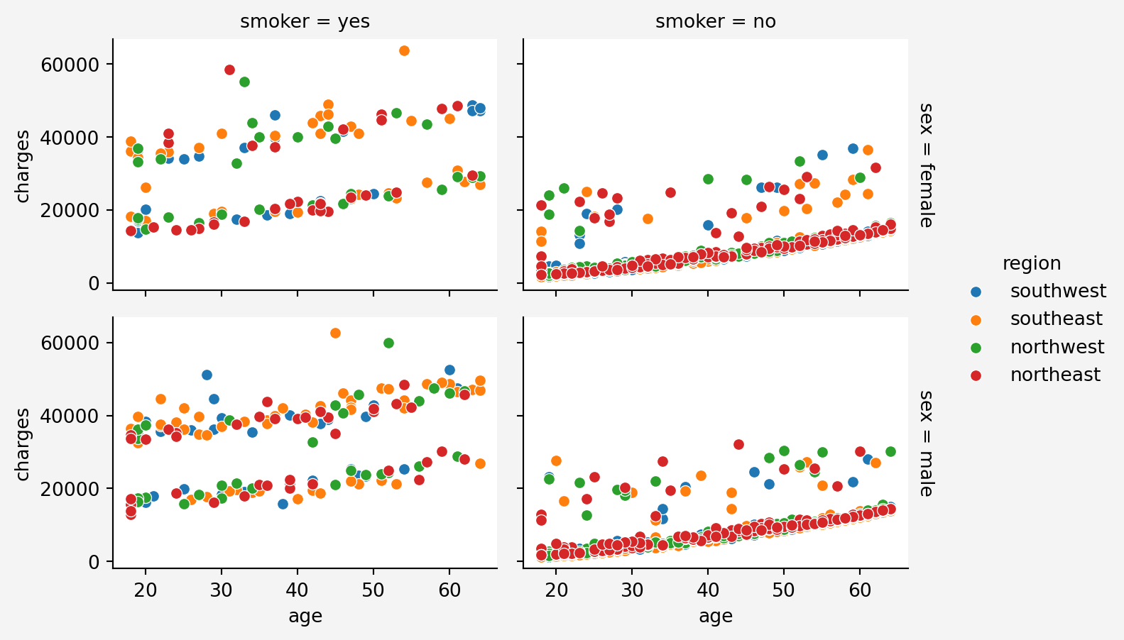
g = sns.FacetGrid(insurance, col='smoker', row='sex',hue='region', margin_titles=True, height=2.4, aspect=1.5)
g.map(sns.scatterplot, 'age','charges')

g.fig.patch.set_facecolor('#f4f4f4')
g.add_legend()
plt.show()

<Figure size 1152x576 with 0 Axes>

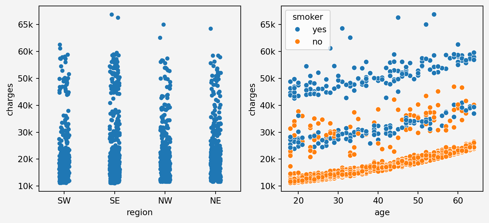
Information Gain

From the above plots, we can see that age feature stacks in three layers for charges. It maybe depending on other categorical features such as smoking status.

Correlation Analysis

Contineous Features

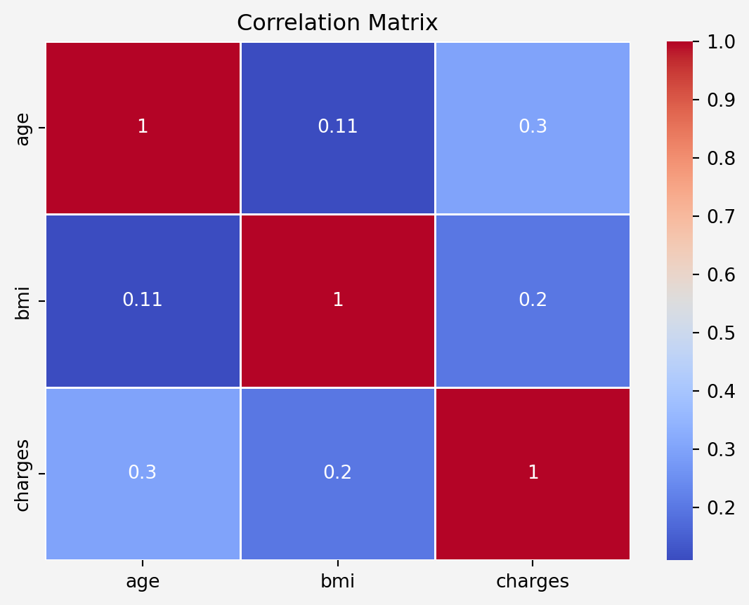
corr_matrix = insurance[['age','bmi','charges']].corr()

sns.heatmap(corr_matrix, annot=True, cmap='coolwarm', linewidths=0.5)
plt.title('Correlation Matrix')
plt.gca().set_facecolor('#f4f4f4') 
plt.gcf().patch.set_facecolor('#f4f4f4')
plt.show()

Categorical Features

import scipy.stats as st
anova_sex, p_value1 = st.f_oneway(
    insurance[insurance['sex']=='male']['charges'],
    insurance[insurance['sex']=='female']['charges']
)

anova_smoker, p_value2 = st.f_oneway(
    insurance[insurance['smoker']=='yes']['charges'],
    insurance[insurance['smoker']=='no']['charges']
)

anova_region, p_value3 = st.f_oneway(
    insurance[insurance['region']=='southwest']['charges'],
    insurance[insurance['region']=='southeast']['charges'],
    insurance[insurance['region']=='northwest']['charges'],
    insurance[insurance['region']=='northeast']['charges']
)

anova_children, p_value4 = st.f_oneway(
    insurance[insurance['children']==0]['charges'],
    insurance[insurance['children']==1]['charges'],
    insurance[insurance['children']==2]['charges'],
    insurance[insurance['children']==3]['charges'],
    insurance[insurance['children']==4]['charges'],
    insurance[insurance['children']==5]['charges']
)

anova_results = {
    'feature_name': ['sex', 'smoker', 'region', 'children'],
    'F-Statistic':[anova_sex, anova_smoker,anova_region,anova_children],
    'p-value':[p_value1, p_value2, p_value3, p_value4]
}

anova = pd.DataFrame(anova_results)
print(anova)

  feature_name  F-Statistic        p-value
0          sex     4.399702   3.613272e-02
1       smoker  2177.614868  8.271436e-283
2       region     2.969627   3.089336e-02
3     children     3.296920   5.785681e-03

Information Gain

Both age and bmi features are positively correlated to charges with correlation coefficients \(0.3\) and \(0.2\), respectively. Since the \(p\)-values are less thatn \(0.05\), therefore, all the categorical features have impact on the target features.

Pre-processing

Data Cleaning

# Binary Encoding for the variables with two categories
from sklearn.preprocessing import LabelEncoder

insurance['male'] = pd.get_dummies(insurance.sex, dtype=int)['male']
insurance['smoke'] = pd.get_dummies(insurance.smoker, dtype=int)['yes']
insurance.drop(['sex','smoker'],axis=1, inplace=True)

label_encoder = LabelEncoder()
insurance['region']=label_encoder.fit_transform(insurance['region'])

new_order = ['age', 'bmi', 'male', 'smoke','children','region', 'charges']
insurance = insurance[new_order]
insurance['charges'] = insurance['charges'].round(2)
insurance.sample(5)

	age	bmi	male	children	region	charges
846	51	34.20	0	1	3	9872.70
290	28	33.40	0	0	3	3172.02
12	23	34.40	1	0	3	1826.84
1285	47	24.32	0	0	0	8534.67
525	18	33.88	0	0	2	11482.63

Check for Multicollinearity

from statsmodels.stats.outliers_influence import variance_inflation_factor

X = insurance.drop('charges', axis=1)
vif_data = pd.DataFrame()
vif_data['feature'] = X.columns
vif_data['VIF'] = [variance_inflation_factor(X.values,i) for i in range(len(X.columns))]
print(vif_data)

    feature        VIF
0       age   7.551348
1       bmi  10.371829
2      male   2.001061
3     smoke   1.256837
4  children   1.801245
5    region   2.924528

Since BMI and Age have higher values for the multicolinearity, therefore we adopt the following methods

Feature Engineering

Interaction term

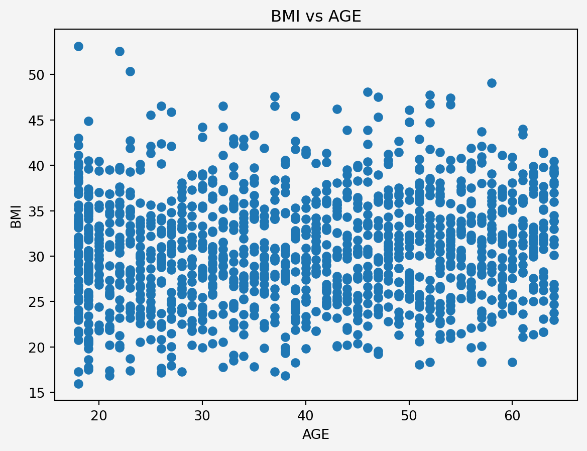
plt.scatter(insurance.age,insurance.bmi)
plt.xlabel('AGE')
plt.ylabel('BMI')
plt.title('BMI vs AGE')
plt.gca().set_facecolor('#f4f4f4') 
plt.gcf().patch.set_facecolor('#f4f4f4')
plt.show()

Since there is no clear linear relationship or any pattern, the Multicollinearity issue can be ignored. However, older individuals with a certain BMI range might have different risks or costs associated with their health. We could explore interaction terms like age * bmi in our model to capture any potential synergistic effects.

insurance.insert(6,'age_bmi',insurance.age*insurance.bmi)
insurance.insert(7,'age_bmi_smoke',insurance.age_bmi*insurance.smoke)
insurance.sample(5,random_state=111)

	age	bmi	male	smoke	children	region	age_bmi	age_bmi_smoke	charges
1000	30	22.99	1	1	2	1	689.70	689.70	17361.77
53	36	34.43	1	1	0	2	1239.48	1239.48	37742.58
432	42	26.90	1	0	0	3	1129.80	0.00	5969.72
162	54	39.60	1	0	1	3	2138.40	0.00	10450.55
1020	51	37.00	1	0	0	3	1887.00	0.00	8798.59

Data Splitting

from sklearn.model_selection import train_test_split
X = insurance.drop('charges',axis=1)
y = insurance['charges'].to_frame()

X_train, X_test, y_train, y_test = train_test_split(
    X, y, test_size=0.30, random_state=42)

Standardization

from sklearn.preprocessing import StandardScaler
from sklearn.compose import ColumnTransformer

conts_features = ['age','bmi','age_bmi']
categ_features = ['male','smoke', 'children','region']

preprocessor = ColumnTransformer(
    transformers=[
        ('num', StandardScaler(), conts_features)
    ],
    remainder= 'passthrough'
)
X_train_sc = preprocessor.fit_transform(X_train)
X_test_sc = preprocessor.fit(X_test)

Model

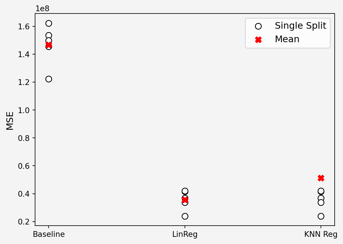
Modelling Approaches

We consider the following models

Baseline model: Assumption that the charges variable can be modeled with the mean value of this charges variable.
\[ \text{charges}=\mathbb{E}[\text{charges}]+\xi \]
Linear Regression with age-bmi-smoke interaction
\[ \text{charges}=\beta_0+\beta_1 (\text{age\_bmi})+\beta_2 (\text{male})+\beta_3 (\text{smoke})+\beta_4 (\text{children})+\beta_5 (\text{region})+\beta_6 (\text{age-bmi-smoke})+\xi \]
K-Neighbor Regression
\(k\)NN using all the original feature

import numpy as np
from sklearn.model_selection import KFold
from sklearn.linear_model import LinearRegression
from sklearn.neighbors import KNeighborsRegressor
from sklearn.metrics import mean_squared_error

kfold = KFold(n_splits=5,shuffle=True, random_state=111)

mses = np.zeros((3,5))

k = 10

for i, (train_index, test_index) in enumerate(kfold.split(X_train_sc)):
    X_train_sc_train = X_train_sc[train_index]
    X_train_sc_holdout = X_train_sc[test_index]

    y_train_train = y_train.iloc[train_index]
    y_train_holdout = y_train.iloc[test_index]

    pred0 = y_train_train.charges.mean()*np.ones(len(test_index))

    model1 = LinearRegression()
    model2 = KNeighborsRegressor(k)

    model1.fit(X_train_sc_train[:,2:], y_train_train)
    model2.fit(X_train_sc_train[:,:6], y_train_train)

    pred1 = model1.predict(X_train_sc_holdout[:,2:])
    pred2 = model2.predict(X_train_sc_holdout[:,:6])


    mses[0,i] = mean_squared_error(y_train_holdout, pred0)
    mses[1,i] = mean_squared_error(y_train_holdout, pred1)
    mses[2,i] = mean_squared_error(y_train_holdout, pred2)

plt.scatter(np.zeros(5), mses[0,:],s=60, c='white', edgecolors='black', label='Single Split')
plt.scatter(np.ones(5), mses[1,:], s=60, c='white', edgecolors='black')
plt.scatter(2*np.ones(5), mses[1,:], s=60, c='white', edgecolors='black')
plt.scatter([0,1,2],np.mean(mses, axis=1),s=60, c='r', marker='X', label='Mean')
plt.legend(loc='upper right', fontsize=12)
plt.xticks([0,1,2],['Baseline','LinReg','KNN Reg'])
plt.yticks(fontsize=10)
plt.ylabel('MSE',fontsize=12)
plt.gca().set_facecolor('#f4f4f4')
plt.gcf().patch.set_facecolor('#f4f4f4')
plt.show()

print(np.mean(np.sqrt(mses),axis=1))
print('\n')
print('Minimum RMSE={} \n Model {}'.format(min(np.mean(np.sqrt(mses),axis=1)),np.argmin(np.mean(np.sqrt(mses),axis=1))) )

[12101.66177575  5938.57275531  7124.33629511]


Minimum RMSE=5938.572755308774 
 Model 1

Final Model

from sklearn.pipeline import Pipeline
from sklearn.base import BaseEstimator, TransformerMixin
from sklearn.preprocessing import OneHotEncoder
data = pd.read_csv('insurance.csv')

class FeatureEngineering(BaseEstimator, TransformerMixin):
    def __init__(self):
        # Initialize OneHotEncoder for 'smoker' and 'sex'
        self.ohe_smoker_sex = OneHotEncoder(
            drop='first', dtype=int, sparse_output=False)
        self.label_encoder = LabelEncoder()

    def fit(self, X, y=None):
        # Fit the OneHotEncoder on smoker and sex
        self.ohe_smoker_sex.fit(X[['smoker', 'sex']])
        self.label_encoder.fit(X['region'])
        return self

    def transform(self, X):
        X = X.copy()

        # Apply OneHotEncoder to 'smoker' and 'sex'
        smoker_sex_encoded = self.ohe_smoker_sex.transform(
            X[['smoker', 'sex']])
        smoker_sex_columns = ['smoker_yes', 'sex_male']

        # Create DataFrame for encoded variables and merge with original data
        smoker_sex_df = pd.DataFrame(
            smoker_sex_encoded, columns=smoker_sex_columns, index=X.index)
        X = pd.concat([X, smoker_sex_df], axis=1)

        # Label encode the 'region' column
        X['region'] = self.label_encoder.transform(X['region'])

        # Create new features
        X['age_bmi'] = X['age'] * X['bmi']
        X['age_bmi_smoker'] = X['age_bmi'] * X['smoker_yes']

        # Drop original columns
        X = X.drop(columns=['age', 'bmi', 'smoker', 'sex'])

        return X

data = pd.read_csv('insurance.csv')
data['charges'] = data['charges'].round(2)

X = data.drop('charges', axis=1)
y = data['charges']

preprocessor = ColumnTransformer(
    transformers=[
        ('scale', StandardScaler(), ['age_bmi', 'age_bmi_smoker'])
    ],
    remainder='passthrough'
)

pipe = Pipeline(steps=[
    ('feature_engineering', FeatureEngineering()),
    ('preprocess', preprocessor),
    ('model', LinearRegression())
])

X_train, X_test, y_train, y_test = train_test_split(
    X, y, test_size=0.3, shuffle=True, random_state=111
)
pipe.fit(X_train, y_train)
print(np.round(pipe['model'].intercept_,2))

10621.25

Model Validation

Root Mean Squared Error (RMSE)

train_prediction = pipe.predict(X_train)
test_prediction = pipe.predict(X_test)

print("Training set RMSE:",
    np.round(np.sqrt(mean_squared_error(train_prediction,y_train)))
)
print("Test set RMSE:",
    np.round(np.sqrt(mean_squared_error(test_prediction,y_test)))
)

Training set RMSE: 5853.0
Test set RMSE: 5600.0

R-Squared (\(R^2\))

from sklearn.metrics import r2_score
y_pred = pipe.predict(X_test)
r2 = r2_score(y_test, y_pred)
print(f'R-squared: {r2:.4f}')

R-squared: 0.8008

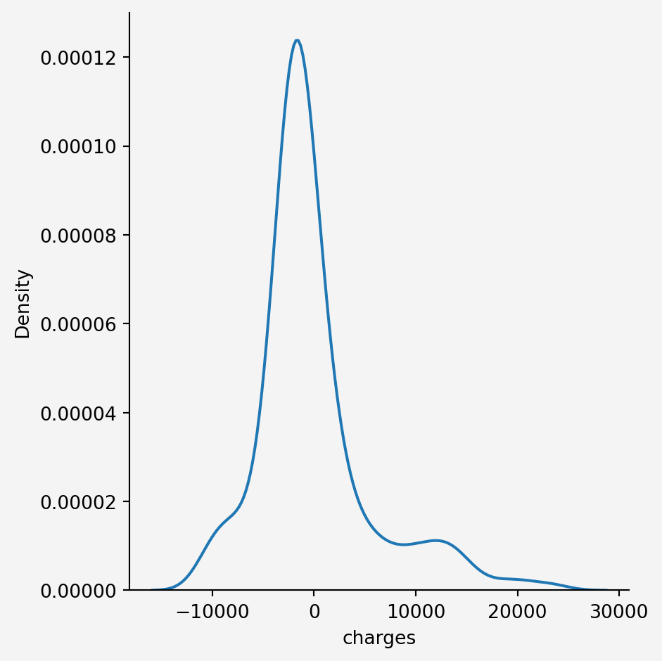
Residuals

res = y_test - y_pred

plt.scatter(y_pred, res)
plt.axhline(y=0, color='r', linestyle='--')
plt.xlabel('Predicted Values')
plt.ylabel('Residuals')
plt.title('Residuals Plot')
plt.gca().set_facecolor('#f4f4f4') 
plt.gcf().patch.set_facecolor('#f4f4f4')
plt.show()

sns.displot(res,kind='kde')
plt.gca().set_facecolor('#f4f4f4') 
plt.gcf().patch.set_facecolor('#f4f4f4')
plt.show()

Development and Deployment

import pickle

pickle.dump(pipe, open('regmodel.pkl','wb'))