K Nearest Neighbors Regression

Introduction: Non-parametric Models

Non-parametric model is a statistical model that does not make any assumptions about the underlying data distributions, meaning it does not require specifying functional form for the relationships between variables, instead learning directly from the data points without pre-defined parameters.

\(K-\)Nearest Neighbors (KNN) Algorithm

K-Nearest Neighbors (KNN) is one of the simplest yet effective algorithms used in supervised learning for both classification and regression problems. It’s a lazy learner—meaning it does not perform any specific training of a model but memorizes the training dataset and makes predictions based on proximity in feature space.

We are given a set of data points \((\bar{x}_i,y_i)\) with \(\bar{x}_i\in \mathbb{R}^d\) and \(y_i\in \mathbb{R}\)
1. Choose the number of neighbors \(K\)
2. Compute the distance between the new data point and all the training samples
3. Select the \(K\) nearest neighbors based on distance.
4. For classification, the output is the most common class among the \(K\) neighbors.
5. For regression, the output is the average of the target values of \(K\) neighbors

\(K-\)Nearest Neighbors Classification

The KNN classification algorithm can be summarized with the following steps:

Given:

• \(X_{train} = [x_1, x_2, \ldots, x_n]\) (the training data features)
  
• \(y_{train} = [y_1, y_2, \ldots, y_n]\) (the training data labels)
  
• \(x_{test}\) (the new data point for which we want to predict the class)

Steps

1. Compute Distance: For each training point \(x_i\), calculate the distance \(d(x_i, x_{test})\) using a distance metric like Euclidean distance: \[ d(x_i, x_{test}) = \sqrt{\sum_{j=1}^{m} (x_{i,j} - x_{test,j})^2} \] where \(m\) is the number of features.

2. Find K Nearest Neighbors: Sort the distances and pick the K closest points.

3. Majority Voting: Look at the labels \(y_i\) of the K nearest neighbors. The predicted label for \(x_{test}\) is the most frequent label (majority vote) among the neighbors.

For example, let’s say our data looks like this

Training Data

area	bedroom	bathroom	price	condition
7420	4	2	1300000	1
7520	3	3	1450000	1
6420	2	1	1110000	0
5423	3	2	1363400	0
5423	3	1	1263400	1

Test Data

area	bedroom	bathroom	price	condition
5420	3	2.5	1302000
7120	5	4	1453000

For the data points \(x_i\) from the training set and a single test data point \(xt=[5420,3,2.5,1302000]\)

\[\begin{align*} d(x_1, xt) & = \sqrt{(x_{11}-xt_1)^2 + (x_{12}-xt_2)^2 + (x_{13}-xt_3)^2 + (x_{14}-xt_4)^2}\\ & = \sqrt{(7420-5420)^2 + (4-5)^2 + (2-2.5)^2 + (1300000-1302000)^2} \approx 2828.43\\ d(x_2,xt) & = \sqrt{(x_{21}-xt_1)^2 + (x_{22}-xt_2)^2 + (x_{23}-xt_3)^2 + (x_{24}-xt_4)^2} \\ & = \sqrt{(7520-5420)^2 + (3-5)^2 + (3-2.5)^2 + (1450000-1302000)^2} \approx 14805.92\\ d(x_3,xt) & = \sqrt{(x_{31}-xt_1)^2 + (x_{32}-xt_2)^2 + (x_{33}-xt_3)^2 + (x_{34}-xt_4)^2} \\ & = \sqrt{(6420-5420)^2 + (2-5)^2 + (1-2.5)^2 + (1110000-1302000)^2} \approx 19209.38\\ d(x_4,xt) & = \sqrt{(x_{41}-xt_1)^2 + (x_{42}-xt_2)^2 + (x_{43}-xt_3)^2 + (x_{44}-xt_4)^2}\\ & = \sqrt{(6420-5420)^2 + (2-5)^2 + (1-2.5)^2 + (1110000-1302000)^2} \approx 19209.38\\ d(x_5,xt) & = \sqrt{(x_{51}-xt_1)^2 + (x_{52}-xt_2)^2 + (x_{53}-xt_3)^2 + (x_{54}-xt_4)^2} \\ & = \sqrt{(5423-5420)^2 + (3-5)^2 + (1-2.5)^2 + (1263400-1302000)^2} \approx 38602.95 \end{align*}\]

So the distances

• \(d_1=d(x_1, xt) \approx 2828.43\)
• \(d_2=d(x_2, xt) \approx 14805.92\)
• \(d_3=d(x_3, xt) \approx 19209.38\)
• \(d_4=d(x_4, xt) \approx 61405.03\)
• \(d_5=d(x_5, xt) \approx 38602.95\)

If we sort the above distances, we get \(d_1<d_2<d_3<d_5<d_4\) and if we choose \(K=3\) nearest neighbors, then \(d_1<d_2<d_3\) and

• Data point \(x_1\) has class label condition\(=1\)
  
• Data point \(x_2\) has class label condition\(=1\)
  
• Data point \(x_3\) has class label condition\(=0\)

We can clearly see that the majority class (2 out of 3) is condition\(=1\). Therefore, for the given test data, the label would be also condition\(=1\).

KNN Classifier Using Python

Here’s how to implement KNN for classification in Python from scratch:

import numpy as np
import pandas as pd
from collections import Counter

class CustomKNNclassifier:

    def __init__(self, k=3):
        self.k = k
    
    def fit(self, X, Y):
        self.X = X
        self.Y = Y
    
    def predict(self, X):
        predictions = [self._predict(x) for x in X.to_numpy()] 
        return np.array(predictions)
    
    def _predict(self, x):
        # Compute the Euclidean distances 
        distances = [np.linalg.norm(x - X_train) for X_train in self.X.to_numpy()]

        # Get the indices of the k nearest neighbors
        k_indices = np.argsort(distances)[:self.k]

        # Get the labels of k nearest neighbors
        k_nearest_neighbors = [self.Y[i] for i in k_indices]

        # Return the most common label
        common_label = Counter(k_nearest_neighbors).most_common(1)[0][0]
        return common_label

# Example usage
train_data = pd.DataFrame(
    {
        'area': [7420, 7520, 6420, 5423, 5423],
        'bedroom': [4, 3, 2, 3, 3],
        'bathroom': [2, 3, 1, 2, 1],
        'price': [1300000, 1450000, 1110000, 1363400, 1263400],
        'condition': [1, 1, 0, 0, 1]
    }
)
test_data = pd.DataFrame(
    {
        'area': [5420, 7120],
        'bedroom': [3, 5],
        'bathroom': [2.5, 4],
        'price': [1302000, 1453000]
    }
)

X_train = train_data.drop('condition', axis=1)
y_train = train_data['condition']

X_test = test_data

# Initialize and train the KNN model
classifier = CustomKNNclassifier(k=3)
classifier.fit(X_train, y_train)

# Predict on test data
predictions = classifier.predict(X_test)
print(predictions)

[1 1]

So the complete test set would be

area	bedroom	bathroom	price	condition
5420	3	2.5	1302000	1
7120	5	4	1453000	1

Note: We did not scale the data before applying the classifier. If we scaled, the result might have been different (?). In practice, we need to scale the data before applying KNN algorithm. Because computing a large number of distances with big numbers may get us wrong order and also time cosuming.

\(K-\)Nearest Neighbors Regression

KNN regression is slightly different from classification. Instead of taking a majority vote, we predict the output by averaging the values of the K nearest neighbors.

Given:

• \(X_{train} = [x_1, x_2, \ldots, x_n]\) (the training data features)
• \(y_{train} = [y_1, y_2, \ldots, y_n]\) (the continuous target values)
• \(x_{test}\) (the new data point for which we want to predict the value)

Step-by-Step:

1. Compute Distance: Calculate the Euclidean distance between \(x_{test}\) and each training point \(x_i\).
2. Find K Nearest Neighbors: Sort the distances and select the K nearest points.
3. Averaging: The predicted value for \(x_{test}\) is the average of the target values \(y_i\) of the K nearest neighbors:

\[ \hat{y}_{test} = \frac{1}{K} \sum_{i=1}^{K} y_i \]

KNN Regressor Using Python

Now we use the same training data and test data for this regression. But this time, our target variable is price and test data looks like this

area	bedroom	bathroom	Condition	price
5420	3	2.5	1
7120	5	4	1

After scaling the data looks like this

Training Data

area	bedroom	bathroom	condition	price
1.213	1.414	0.267	0.730	1300000
1.336	0.000	1.603	0.730	1450000
-0.026	-1.414	-1.336	-1.095	1110000
-1.261	0.000	0.267	-1.095	1363400
-1.261	0.000	-1.336	0.730	1263400

Test Data

area	bedroom	bathroom	condition	price
-1.266	0.000	0.803	0.730
0.854	2.828	3.876	0.730

Now we see that

\[\begin{align*} d_1=d(x_1, x_t) & = \sqrt{(1.213 - (-1.266))^2 + (1.414 - 0)^2 + (0.267 - 0.803)^2 + (0.730 - 0.730)^2} \approx 2.904\\ d_2=d(x_2, x_t) & = \sqrt{(1.336 - (-1.266))^2 + (0.000 - 0)^2 + (1.603 - 0.803)^2 + (0.730 - 0.730)^2} \approx 2.721\\ d_3=d(x_3, x_t) & = \sqrt{(-0.026 - (-1.266))^2 + (-1.414 - 0)^2 + (-1.336 - 0.803)^2 + (-1.095 - 0.730)^2} \approx 3.382\\ d_4=d(x_4, x_t) & = \sqrt{(-1.261 - (-1.266))^2 + (0.000 - 0)^2 + (0.267 - 0.803)^2 + (-1.095 - 0.730)^2} \approx 1.902\\ d_5=d(x_5, x_t) & = \sqrt{(-1.261 - (-1.266))^2 + (0.000 - 0)^2 + (-1.336 - 0.803)^2 + (0.730 - 0.730)^2} \approx 2.140 \end{align*}\]

But this time, the order is \(d_4<d_5<d_2<d_1<d_3\) and for \(k=3\) we have \(d_4<d_5<d_2\). The price for this distances

• For data point \(x_4\), the price\(=1363400\)
  
• For data point \(x_5\), the price\(=1263400\)
  
• For data point \(x_2\), the price\(=1450000\)

So the predicted price should be the average of this three prices, that for \(xt=[5420,3,2.5,1]\) the price we expect
\[ price = \frac{1363400+1263400+1450000}{3}=1358933.33 \]

Here’s how to implement KNN for regression in Python from scratch and we see if we get the same as the hand calculation.

from sklearn.preprocessing import StandardScaler

class CustomKNNRegressor:
    def __init__(self, k=3):
        self.k = k

    def fit(self, X_train, y_train):
        self.X_train = X_train
        self.y_train = y_train.to_numpy()

    def predict(self, X_test):
        predictions = [self._predict(x) for x in X_test]
        return np.array(predictions)
    
    def _predict(self, x):
        distances = [np.linalg.norm(x-x_train) for x_train in self.X_train]
        k_indices = np.argsort(distances)[:self.k]
        k_nearest_values = [self.y_train[i] for i in k_indices]
        return np.mean(k_nearest_values)

X_train = train_data.drop('price', axis=1)
y_train = train_data['price']

test_data = pd.DataFrame(
    {
        'area': [5420, 7120],
        'bedroom': [3, 5],
        'bathroom': [2.5, 4],
        'condition': [1, 1]
    }
)

X_test = test_data

scaler = StandardScaler()

X_train_sc = scaler.fit_transform(X_train)
X_test_sc = scaler.transform(X_test)

# Initialize and train the KNN regressor
regressor = CustomKNNRegressor(k=3)
regressor.fit(X_train_sc, y_train)

# Predict on test data
predictions = regressor.predict(X_test_sc)
print(np.round(predictions,2))

[1358933.33 1371133.33]

---

Choosing the Value of K

The value of K significantly affects the performance of the KNN algorithm:

• Small K: If K is too small, the model is sensitive to noise, and the predictions can be unstable.
  
• Large K: If K is too large, the model becomes more biased, and the predictions may be overly smoothed.

A typical way to choose K is by trying different values and using cross-validation to see which value yields the best performance.

---

Distance Metrics

The default metric for KNN is Euclidean distance, but depending on the dataset, other metrics like Manhattan distance or Minkowski distance might be more suitable.

• Euclidean Distance (L2 Norm): \[ d(x_i, x_j) = \sqrt{\sum_{k=1}^{m} (x_{i,k} - x_{j,k})^2} \]

• Manhattan Distance (L1 Norm): \[ d(x_i, x_j) = \sum_{k=1}^{m} |x_{i,k} - x_{j,k}| \]

KNN Implementation

In this section we use KNN regression for Boston Housing dataset and find the optimal \(K\) using the KFold cross-validation.

df = pd.read_csv('HousingData.csv')

Next we see if there is any missing values. If we have any, we will skip those observations.

print(df.isnull().sum())
df.dropna(axis=1,inplace=True)
df.head()

CRIM       20
ZN         20
INDUS      20
CHAS       20
NOX         0
RM          0
AGE        20
DIS         0
RAD         0
TAX         0
PTRATIO     0
B           0
LSTAT      20
MEDV        0
dtype: int64

	NOX	RM	DIS	RAD	TAX	PTRATIO	B	MEDV
0	0.538	6.575	4.0900	1	296	15.3	396.90	24.0
1	0.469	6.421	4.9671	2	242	17.8	396.90	21.6
2	0.469	7.185	4.9671	2	242	17.8	392.83	34.7
3	0.458	6.998	6.0622	3	222	18.7	394.63	33.4
4	0.458	7.147	6.0622	3	222	18.7	396.90	36.2

The data looks clean and ready to implement to the KNNRegressor. Note that, for predictive modeling we need a lot of things, such as exporatory data analysis (EDA), feature engineering, preprocessing and others. However, we will simply apply the KNNRegressor that we built from scratch and built-in library function from scikit-learn to explore the algorithm and find the optimal \(K\).

from sklearn.model_selection import KFold, train_test_split
from sklearn.metrics import mean_squared_error,r2_score
import matplotlib.pyplot as plt 


X = df.drop('MEDV',axis=1)
y = df['MEDV']

X_train, X_test, y_train, y_test = train_test_split(
    X,y, test_size=0.30, random_state=123
)
scaler = StandardScaler()
X_train_sc = scaler.fit_transform(X_train)
X_test_sc = scaler.transform(X_test)

k_values = [5,15,30,40]

kfold = KFold(n_splits=7, shuffle=True, random_state=123)
mses = np.zeros((7,4))

for i,(train_index,test_index) in enumerate(kfold.split(X_train_sc)):
    X_train_train = X_train_sc[train_index]
    X_train_holdout = X_train_sc[test_index]

    y_train_train = y_train.iloc[train_index]
    y_train_holdout = y_train.iloc[test_index]

    for j,k in enumerate(k_values):
        regressor1 = CustomKNNRegressor(k=k)
        regressor1.fit(X_train_train, y_train_train)
        preds = regressor1.predict(X_train_holdout)
        mses[i,j] = mean_squared_error(preds, y_train_holdout)

plt.scatter(np.zeros(7),mses[:,0], s=60, c='white', edgecolors='black', label='Single Split')
plt.scatter(np.ones(7),mses[:,1],s=60, c='white', edgecolors='black')
plt.scatter(2*np.ones(7),mses[:,2],s=60, c='white', edgecolors='black')
plt.scatter(3*np.ones(7),mses[:,3],s=60, c='white', edgecolors='black')
plt.scatter([0,1,2,3], np.mean(mses, axis=0), s=60,c='r', marker='X', label='Mean')
plt.legend(loc='upper right')
plt.xticks([0,1,2,3],['K=5','K=15','K=30','K=40'])
plt.ylabel('MSE')
plt.gca().set_facecolor('#f4f4f4')
plt.gcf().patch.set_facecolor('#f4f4f4')
plt.show()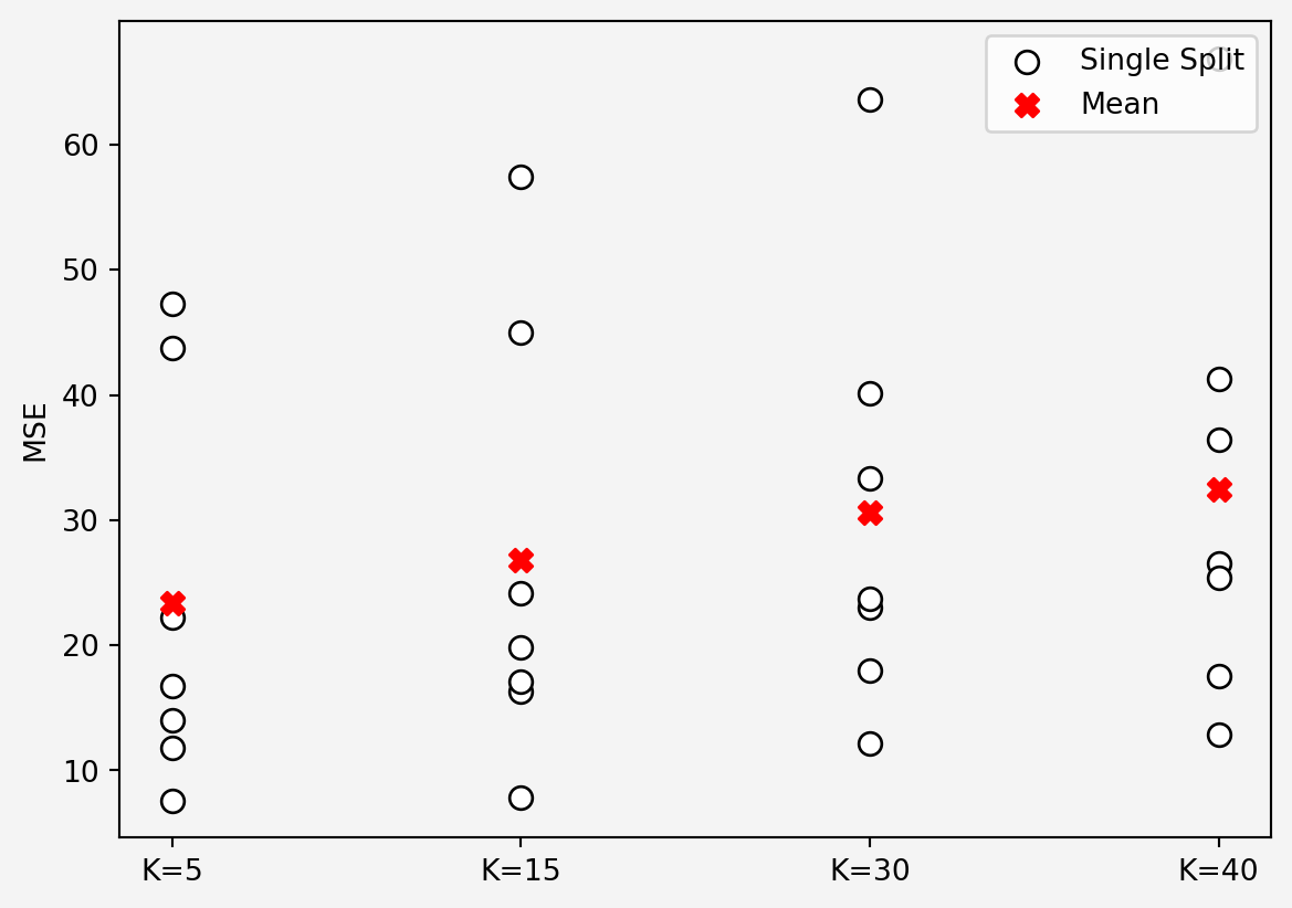

So, \(K=5\) seems optimal based on our custom built regressor. Now if we do the same thing using the scikit-learn library

from sklearn.neighbors import KNeighborsRegressor


mses = np.zeros((7,4))

for i,(train_index,test_index) in enumerate(kfold.split(X_train_sc)):
    X_train_train = X_train_sc[train_index]
    X_train_holdout = X_train_sc[test_index]

    y_train_train = y_train.iloc[train_index]
    y_train_holdout = y_train.iloc[test_index]

    for j,k in enumerate(k_values):
        regressor2 = KNeighborsRegressor(k)
        regressor2.fit(X_train_train, y_train_train)
        preds = regressor2.predict(X_train_holdout)
        mses[i,j] = mean_squared_error(preds, y_train_holdout)

plt.scatter(np.zeros(7),mses[:,0], s=60, c='white', edgecolors='black', label='Single Split')
plt.scatter(np.ones(7),mses[:,1],s=60, c='white', edgecolors='black')
plt.scatter(2*np.ones(7),mses[:,2],s=60, c='white', edgecolors='black')
plt.scatter(3*np.ones(7),mses[:,3],s=60, c='white', edgecolors='black')
plt.scatter([0,1,2,3], np.mean(mses, axis=0), s=60,c='r', marker='X', label='Mean')
plt.legend(loc='upper right')
plt.xticks([0,1,2,3],['K=5','K=15','K=30','K=40'])
plt.ylabel('MSE')
plt.gca().set_facecolor('#f4f4f4')
plt.gcf().patch.set_facecolor('#f4f4f4')
plt.show()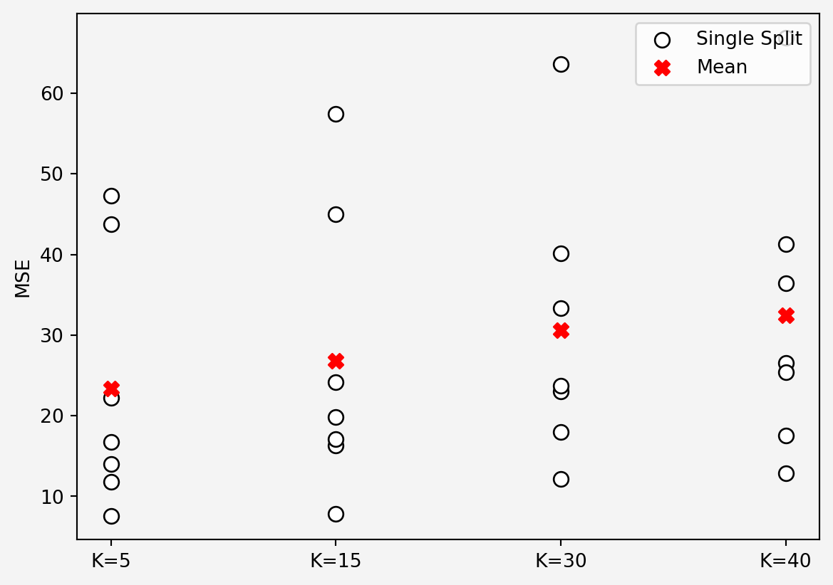

In both method, we got \(K=5\) is the optimal number of neighbors for KNN regression. Let’s apply this in our test dataset

regressor = CustomKNNRegressor(k=5)
regressor.fit(X_train_sc, y_train)

predictions = regressor.predict(X_test_sc)

mse = mean_squared_error(predictions,y_test)
rsquared = r2_score(predictions,y_test)
print('MSE = {}'.format(np.round(mse,2)),' and R-square = {}'.format(np.round(rsquared,2)))

MSE = 41.26  and R-square = 0.23

Conclusion

K-Nearest Neighbors is a simple, intuitive algorithm that can be highly effective in both classification and regression problems. Its simplicity comes from the fact that it doesn’t make any assumptions about the underlying data distribution (it’s non-parametric). However, its performance can be sensitive to the choice of K and the distance metric.

Although it’s easy to implement, KNN can become computationally expensive for large datasets, as it requires calculating distances between the test point and all training samples.

If you need an efficient version, it’s always possible to use optimized libraries like scikit-learn, but writing the algorithm from scratch helps build a solid understanding.

When to Use KNN Over Linear Regression?

We would consider using KNN regression over linear regression in the following situations:

• Non-linear relationships: When the data shows non-linear patterns or complex relationships between features and target variables that cannot be captured by a straight line.
  
• Local behavior: When data has local patterns or clusters, and you believe that predictions should rely on the nearest data points.
  
• Minimal assumptions: If you do not want to assume a specific relationship between the features and target, KNN’s non-parametric nature might be more appropriate.
  
• Smaller datasets: KNN works well with smaller datasets and lower-dimensional data where calculating distances is feasible and efficient.

However, KNN becomes less efficient and struggles in high dimensions or when the dataset is large. In those cases, linear regression or other more scalable models may be more appropriate

---

References

1. KNN Regressor Overview:
   • Géron, Aurélien. Hands-On Machine Learning with Scikit-Learn, Keras, and TensorFlow: Concepts, Tools, and Techniques to Build Intelligent Systems. O’Reilly Media, 2019. This book provides an in-depth explanation of KNN, including its behavior in non-linear data and high-dimensionality challenges.
   • Bishop, Christopher M. Pattern Recognition and Machine Learning. Springer, 2006. This book covers non-parametric methods like KNN, highlighting the “curse of dimensionality” and distance-based approaches.
2. KNN vs. Linear Regression (Model Assumptions & Complexity of Data):
   • Hastie, Trevor, Tibshirani, Robert, and Friedman, Jerome. The Elements of Statistical Learning: Data Mining, Inference, and Prediction. Springer, 2009. This source discusses the assumptions behind linear regression and the flexibility of non-parametric models like KNN.
   • Kuhn, Max, and Johnson, Kjell. Applied Predictive Modeling. Springer, 2013. The comparison between parametric (like linear regression) and non-parametric models (like KNN) is elaborated in this book.
3. Interpretability:
   • Molnar, Christoph. Interpretable Machine Learning: A Guide for Making Black Box Models Explainable. 2019. This book emphasizes the trade-offs between interpretable models like linear regression and more black-box models like KNN.
   • Murdoch, W. James, et al. “Definitions, methods, and applications in interpretable machine learning.” Proceedings of the National Academy of Sciences 116.44 (2019): 22071-22080.
4. Sensitivity to Outliers:
   • Aggarwal, Charu C. Data Classification: Algorithms and Applications. Chapman and Hall/CRC, 2014. This discusses the impact of outliers on different models, including linear regression and KNN.
   • Friedman, Jerome, et al. The Elements of Statistical Learning. Springer Series in Statistics, 2001. Sensitivity to outliers is compared across various regression techniques, including KNN.
5. Handling High-Dimensional Data:
   • Domingos, Pedro. “A few useful things to know about machine learning.” Communications of the ACM 55.10 (2012): 78-87. This paper discusses challenges like the curse of dimensionality in models like KNN.
   • Verleysen, Michel, and François, Damien. “The curse of dimensionality in data mining and time series prediction.” International Work-Conference on Artificial Neural Networks. Springer, 2005.
6. Training and Prediction Time:
   • Shalev-Shwartz, Shai, and Ben-David, Shai. Understanding Machine Learning: From Theory to Algorithms. Cambridge University Press, 2014. Provides insights into the computational cost differences between linear and non-parametric models like KNN.
   • Li, Zhe, et al. “Fast k-nearest neighbor search using GPU.” International Conference on Image and Graphics. Springer, 2015. This paper discusses computational complexity related to KNN.
7. Overfitting and Flexibility:
   • Yao, Ying, et al. “Overfitting and Underfitting: A Visual Explanation.” Towards Data Science, 2019. Offers a visual and intuitive explanation of the bias-variance tradeoff in KNN and linear models.
   • Rasmussen, Carl E., and Williams, Christopher KI. Gaussian Processes for Machine Learning. MIT Press, 2006. Discusses overfitting in KNN due to small values of k and regularization techniques for linear models.

---

Share on

You may also like